Search & Planning

Introduction to AI (I2AI)

Andy Weeger

Neu-Ulm University of Applied Sciences

March 12, 2025

Introduction

Planning agents

Rational agents select actions to maximize performance across time.

Planning involves mapping action sequences from current to goal states.

Solutions for search problems are efficient action sequences reaching goal states.

Optimization differs from planning—focuses on finding optimal states, not paths.

Examples

Terms

Agents that plan by considering a sequence of actions that form a path to a goal are called planning agents (Russel and Norvig 2022, 81).

The computational process it undertakes is search.
The representations the agents use are atomic representations¹.
The search algrotihms can be uninformed and informed.

Here only simple environments are considered (episodic, single agent, fully observable, deterministic, static, discrete, and known).

We assume that information about the environment are given (e.g., a map)

Problem-solving process

In simple environments, agents can follow a four-phase-problem-solving process (Russel and Norvig 2022, 81–82):

Goal formulation: Identifying the objectives to be achieved based on the current situation and agent’s purpose
Problem formulation: Deciding what states and actions to consider to achieve the goal²
Search: Systematically exploring possible sequences of actions to find a solution path from initial state to goal state
Execution: Carrying out the solution actions in the environment

Search problem

Definition

A search problem can be defined formally as (Russel and Norvig 2022, 83):

State space: a set of possible states³ the environment can be in⁴
Initial state: the state that the agent starts
Goal state(s): a state that the agent is trying to reach⁵
Transition model: \(\textrm{RESULT}(s,a)\) — returns the state \(s'\) that results from performing action \(a\) in state \(s\)
Successor function: \(\textrm{ACTIONS}(s)\) — returns a set of (action, state) pairs for node \(s\), where the state is the state reachable by taking the action \(a\)
Action cost function: \(\textrm{ACTION-COST}(s,a,s')\) — gives the numeric cost of performing action \(a\) in state \(s\) to reach state \(s'\)
Path: a sequence of actions
Solution: a path from the initial state to the goal state

Examples

Navigation

State space: All possible waypoints (intersections, landmarks) in the road network
Initial state: Starting waypoint of the agent (e.g., home intersection, current street position)
Goal state(s): Destination waypoint(s) the agent wants to reach (e.g., store intersection, airport terminal entrance)
Transition model: Model that returns the new waypoint after traveling along a specific road segment
Successor function: Model that returns available road segments (streets, highways) and resulting waypoints connected to current waypoint
Action cost function: Model that returns the distance, time, or fuel consumption for traveling between waypoints (maybe influenced by speed limits, traffic, road conditions)
Path: A sequence of road segments through the network
Solution: A sequence of road segments from starting waypoint to destination waypoint

8-Puzzle

State space: All possible configurations of the 8 numbered tiles in a 3×3 grid (with one empty space)
Initial state: Starting arrangement of tiles (a specific configuration of the 8 tiles and empty space)
Goal state(s): Target arrangement of tiles (typically tiles in numerical order with empty space in a specific position)
Transition model: Model that returns the new configuration after sliding a tile into the empty space
Successor function: AModel that returns possible slides (up, down, left, right) of adjacent tiles into the empty space and resulting configurations
Action cost function: Typically uniform cost of 1 per move
Path: A sequence of tile slides
Solution: A sequence of tile slides from initial configuration to goal configuration

Chess

State space: All possible legal board configurations of chess pieces
Initial state: Standard starting position with all pieces in their traditional positions
Goal state(s): Any board configuration where the opponent’s king is in checkmate
Transition model: Model that returns the new board configuration after making a specific move
Successor function: AModel that returns all legal moves and resulting board configurations from current position
Action cost function: Typically uniform cost of 1 per move
Path: A sequence of chess moves
Solution: A sequence of moves from the initial position to a checkmate position

Problem formulation (modelling)

Figure 1: Example: A simplified map of Romania, with road distances in miles; based on Russel and Norvig (2022, 84)

Figure 1 depicts the search problem as model, the state space graph:

State space: cities (vertices, each state occurs only once)
Initial state: Arad
Goal state: Bucharest (goal test: \(Is state == Bucharest?\))
Actions: directed edges between the vertices (paths)
Action costs: numbers on the paths

Modelling & abstraction

The model is an abstract mathematical description, here a simple atomic state description. The model is an abstraction as it ignores many details of the reality (e.g., weather and scenery).

Modeling as a process includes:

Deciding which aspects of the real-world problem are relevant
Choosing appropriate abstractions and simplifications
Determining the right level of granularity (e.g., waypoints vs. coordinates)
Making assumptions about the problem domain
Selecting the suitable problem-solving paradigm (search, constraint satisfaction, optimization, etc.)

A good problem formulation has the right level of detail (i.e., an appropriate level of abstraction).

The choice of a good abstraction involves removing as much detail as possible while retaining validity and ensuring that the abstract actions are easy to carry out. An abstraction is valid if any abstract solution can be elaborated into a solution in the more detailed world.

Search trees

Definition

The formulation of a search problem, encompassing the definition of state space, initial state, goal states, transition model, and other pertinent elements, effectively constitutes the blueprint for a search tree:

The root node of the tree corresponds to your initial state
The branches represent actions defined by your transition model
The child nodes are states resulting from taking those actions
Leaf nodes are states with no successors (or states we choose not to expand)
Goal nodes are states that satisfy your goal condition

The search tree is the computational manifestation of your problem formulation.

The quality of your your problem formulation directly affects:

The structure of the tree (branching factor, depth)
The efficiency of search algorithms traversing it
The quality of solutions found

For example, in the 8-puzzle problem, a poor modeling choice might represent the entire board as a single entity, while a better model would represent each tile position individually, resulting in a more manageable search tree.

Modelling choice examples

Continuous coordinate system modeling approach

If we model navigation using precise GPS coordinates (latitude/longitude): - States would be exact positions: (37.7749, -122.4194) - Actions would be small movements in any direction - Transition model would calculate new coordinates based on direction and distance

This approach creates problems:

Enormous state space: infinite possible positions
Unrealistic movement model: doesn’t account for road constraints
Inefficient search: most coordinates don’t correspond to valid paths
Complex cost calculation: difficult to determine if movement between coordinates is even possible

Waypoint graph modeling approach

A better approach models the problem as a graph of waypoints:

States: discrete locations (intersections, landmarks): node_123
Actions: road segments connecting waypoints: take_main_street
Transition model: graph edges showing direct connections
Cost function: actual road distances, travel times, or other metrics

Benefits of this approach:

Drastically reduced state space: only meaningful locations are represented
Realistic movement model: only follows actual roads
Efficient search: branching factor limited to connected roads
Accurate cost calculation: based on real road metrics (distance, speed limits, traffic)

The waypoint model transforms an infinite continuous problem into a finite discrete one, making the search tree dramatically smaller and focused only on relevant states. This allows standard search algorithms like A* to efficiently find optimal routes in reasonable time frames, even for large maps.

Frontier

The frontier (sometimes called the “open list” or “fringe”) is the collection of nodes that have been generated but not yet expanded or evaluated.

The frontier serves as the boundary between explored and unexplored parts of the search space. It contains all the nodes that are immediate candidates for expansion.

You might also call the frontier the “to-do list” of nodes that the search algorithm maintains.

Example

Figure 2: Example: A partial search tree for finding a route from Arad to Bucharest; based on Russel and Norvig (2022)

Figure 2 visualizes a partial search tree: the first few steps in finding a path from Arad (initial state) to Bucharest (goal).

The root node of the search tree is the initial state \(s\) (Arad)
The available actions per state can be queried using \(ACTIONS(s)\)
The current node is expanded by generating child nodes or successor nodes using the available actions and \(RESULT(s,a)\)
Each resulting child node has Arad as its parent node
The frontier contains all not yet expanded nodes
The child node to be considered next is selected by the minimum value of some evaluation function \(f(n)\)

In Figure 2, nodes that have been expanded are white with bold letters; nodes on the frontier that have been generated but not yet expanded are in white and regular letters; the set of states corresponding to these two types of nodes are said to have been reached. Nodes that could be generated next are shown in faint dashed lines.

Definition of search trees

A search tree is a “what if” tree of plans and their outcomes.

The start state is the root node,
children correspond to successors,
nodes show states, but correspond to PLANS that achieve those states

There are lots of repeated structure in the search tree. Thus, for most problems, the whole tree can never be actually built. In practice, both state space graphs and search trees are constructed on demand and as little as possible (Russel and Norvig 2022).

Search algorithms require a data structure to keep track of the search tree. A node in the tree is represented by a data structure with four components (Russel and Norvig 2022, 91):

node.STATE: the state to which the node corresponds
node.PARENT: the node in the tree that generated this node
node.ACTION: the action that was applied to the parent’s state to generate this node
node.PATH-COST: the total cost of the path from the initial state to generate this node

Following the PARENT pointers back from a node allows to revocer the states and actions along the path to that node. Doing this from a goal node generates the solution.

Example data structure in pseudo code

var searchTree = {
  node.STATE: "Bucharest"
  node.PARENT: {
    node.STATE: "Pitesti"
    node.PARENT: {
      node.STATE: "Rimmicu Vilcea"
      node.PARENT: {
        node.STATE: "Sibiu"
        node.PARENT: {
          node.STATE: "Arad"
          node.PARENT: NULL
          node.ACTION: NULL
          node.PATH-COST: 0
        }
        node.ACTION: "Arad to Sibiu"
        node.PATH-COST: 140
      }
      node.ACTION: "Sibiu to Rimmicu Vilcea"
      node.PATH-COST: 220
    }
    node.ACTION: "Rimmicu Vilcea to Pitesti"
    node.PATH-COST: 317
  }
  node.ACTION: "Pitesti to Bucharest"
  node.PATH-COST: 418
}

In addition, a data structure to store the frontier is neded. Usually this is realized using a queue with following functions (Russel and Norvig 2022, 91):

IS-EMPTY(frontier): returns true only if there are no nodes in the frontier
POP(frontier): removes the top node from the frontier and returns it
TOP(frontier): returns (but does not remove) the top node from the frontier
ADD(node,frontier): inserts node into its proper place in the queue

Search algorithms

Definition

Search algorithms take a search problem as input and return a solution, or an indication of failure (Russel and Norvig 2022, 89).

They superimpose a search tree over the state-space graph,
form various paths from the initial state, and
try to find a path that reaches a goal state.

Depending on the problem formulation, they can implement different methods:

Uninformed search, which only have access to the problem definition but not clue about how close a state is to the goal(s).
Informed search, which have access to a heuristic function that gives domain-specific hints about how close a state is to the goal(s) (e.g., using straight-line distance in route-finding problems)

Performance metrics

Performance metrics guide the choice of algorithms based on problem requirements, help predict computational demands, and establish clear expectations about what an algorithm can and cannot do.

Completeness refers to an algorithm’s guarantee to find a solution.
Optimality refers to the algorithm’s capability to find the optimal solution.
Complexity determines time and memory/space requirements.
Global solutions (path) vs. local solutions (optimal or satisfactory state only).

Completeness refers to an algorithm’s guarantee to find a solution if one exists, ensuring that no potential solution path is overlooked during the search process. This property is crucial in critical applications where finding any viable solution is mandatory, such as medical diagnosis systems or emergency response planning, as it provides certainty that the algorithm won’t fail by getting stuck in infinite loops or dead ends.

Optimality ensures that an algorithm will find not just any solution, but the best possible one according to a defined cost function, whether that’s shortest distance, minimum time, lowest energy consumption, or other metrics. This property is essential in resource-constrained environments where efficiency matters significantly, such as route planning, supply chain optimization, or bandwidth allocation, as it guarantees maximum value from available resources.

Complexity measures how an algorithm’s resource requirements (time and memory) scale with increasing problem size, typically expressed using big O notation in terms of factors like branching factor and solution depth. Understanding complexity helps predict whether an algorithm will be practically usable for real-world problems or if it will exceed available computational resources, making it a critical consideration when deploying algorithms in time-sensitive applications or on hardware with limited capabilities.

Global solutions provide a complete path from initial state to goal state, offering step-by-step instructions for transitioning between states, whereas local solutions focus only on finding an optimal or good state without specifying how to reach it. This distinction is important because global solution algorithms (like A* or BFS) are essential for navigation and planning tasks requiring explicit paths, while local solution approaches (like hill climbing or genetic algorithms) can be more efficient for optimization problems where only the final configuration matters, not the route taken to achieve it.

Uninformed search

Figure 3: Overview of uninformed search strategies

Greedy best-first search

The Greedy best-first search uses the evlation function \(f(n) = h(n)\)

It expands the first node with the lowest \(h(n)\) value in the queue.

In route finding problems, the straight-line distance heuristic is used as \(h(n)\).

Greedy best-first graph search is complete in finite state spaces, but not in infinite ones.

A* Search

The A* search (pronounced “A-star search”) uses the evaluation function \(f(n) = g(n) + h(n)\).

\(g(n)\) is the path cost from the initial state to node \(n\) (e.g., computed by using the action-cost function).
\(h(n)\) is the estimated cost of the shortes path from \(n\) to a goal state.

A* search is complete, if it is cost-optimal depends on the heuristic.

Online search

The agents considered so far use offline search algorithm. They compute a complete solution before taking their first action. They are not helpful in unknown environments.

Online search agents interleaves computation and action:

Takes action,
observes the environment, and
computes the next action,

These agents can discover successor only for a state that is occupied or that is learned (i.e., contained in a map created online)

Online search is a good idea in dynamic or semi-dynamic environments.

2-Player games

Example: AlphaGo

AlphaGo is a computer program that plays the board game Go, which is considered much more difficult for computers to win than other games such as chess because its strategic and aesthetic nature makes it difficult to construct a direct scoring function. AlphaGo was developed by the London-based DeepMind Technologies, an acquired subsidiary of Alphabet Inc.

Figure 4: A human trying to beat AlphaGo

AlphaGo use a Monte Carlo tree search algorithm to find their moves based on knowledge previously acquired through machine learning, specifically an artificial neural network (a deep learning method) through extensive training, both from human and computer games. A neural network is trained to recognize the best moves and the winning rates of those moves. This neural network improves the strength of the tree search, leading to stronger move selection in the next iteration. It is used to decide on

the next action to choose in the selection-phase,
which leaf-node to extend in the expansion phase, and
which actions to choose in the simulation phase

A nice summary of MCTS and AlphaGo can be found here.

Adversarial search

In competitive environments, two or more agents have conflicting goals, which gives rise to adversarial search problems.

The algorithm described in this section is applicable for all games with the following characteristics:

2 players fully observable deterministic zero-sum

As in such games the state of a game is easy to represent, agents are restricted to a few actions and effects of actions are defined by precise rules (Russel and Norvig 2022, 192).

MinMax value

Given a state-space search tree, each node’s MinMax value is calculated.

The MinMax value is the best achievable utility of being in a given sate (against a rational adversary).

MAX prefers to move to a state of maximum value
MIN prefers to move to a state of minimum value

Adversarial game tree

MinMax algorithm

The MinMax algorithm performs a complete depth-first exploration of the game tree (Russel and Norvig 2022, 196–96).

Assumes that the adversary plays optimal.
Returns action whose terminal state has the optimal MinMax value.
The tree is calculated down to a maximum depth \(L\) (i.e., the planning horizon).
If level \(L-1\) belongs to Min MinMax will choose in each state the action, which leads to a successor of minimum utility — since minimum utility for Max is maximum utility of Min. Therefore, to each node in level \(L-1\), the minimum utility of it’s successor nodes is assigned.
In the same way to each node in level \(L-2\), the maximum utility of it’s successor nodes in level \(L-1\) is assigned.
This process is repeated up to the root node. Max then knows his next action — the one, which yields to a successor with maximum utility-value.

Alpha-Beta Pruning

Alpha-Beta Pruning is an improvement of the MinMax algorithm in the sense that it reduces the number of nodes, that have to be evaluated and generated by applying a simple logic (Russel and Norvig 2022, 198–99). The process is as follows:

Create tree with limited depth search from left to right
As in MinMax-search evaluate nodes in the deepest level by applying a domain-specific evaluation function
For each Max-node store the maximum value of the underlying subtree traversed so far in the variable
For each Min-node store the minimum value of the underlying subtree traversed so far in the variable
If at a minimum node \(k\) the current value β is smaller than α the search under \(k\) can be terminated. Here α is the largest value of a maximum node in the path from the root to \(k\).
If at a maximum node k the current value α is larger than β, the search under \(k\) can be terminated. Here β is the smallest value of a minimum node in the path from the root to \(k\).

A nice simulation of MinMax- and AlphaBeta-Pruning can be found here.

Why Alpha-Beta

Pruning stops the search at the moment when it is determined that the value of a subtree is worse than the best solution already identified. Alpha-beta pruning gets its name from the two extra parameters in MAX-VALUE(state,α,β) that describe the bounds on the backed-up values that appear anywhere along the path:

α = the value of the best choice for MAX found so far (“at least”)
β = the value of the bast choice for MIN found so far (“at most”)

Alpha-beta search updates the values of α and β as it goes along and prunes the remaining branches at a node as soon as the value of the current node is known to be worse than the current α and β for MAX or MIN, respectively (Russel and Norvig 2022, 198).

Monte Carlo tree search

Introduction

The concept of a limited planning horizon, as applied in the MinMax-algorithm is one way to handle complex problems, which can not be planned to the goal-state in one step.

Another concept is to construct a tree until a final state in such a way that in each state only promising actions and corresponding successors are generated. This concept is applied by Monte Carlo tree search.

Functioning

Monte Carlo tree search (MCTS)⁹ does estimate the value of a state as the average utility¹⁰ over a number of simulations of complete games starting from the current state (Russel and Norvig 2022, 207–9).

Each iteration follows four steps:

Selection: starting from the root node, apply tree policy in order to select next action (e.g., based on average utility¹¹).
Expansion: in a leaf-node select an arbitrary action and generate the corresponding new child-node.
Simulation: simulate the game, starting from the new child-node. At the end of each simulation the game is won or lost.
Backpropagation: the result of the simulation is used to update all the search tree nodes going up to the root.

If the computational budget is reached, MCTS returns with the best action a for the given root node.

Example: selection

Figure 6 shows a tree with the root representing a state where P-A has won 37/100 playouts done

P-A has just moved to the root node
P-B selects a move to a node where it has won 60/79 playouts; this is the best win percentage among the available moves
P-A will select a move to a node where it has won 16/53 playouts (assuming it plays optimally)
P-B then continues on the leaf node marked 27/35
… until a terminal state is reached

Example: selection policy (UCT)

Upper confidence bounds applied to trees (UCT) is a very effective selection policy ranking possible moves based on an upper confidence bound formula (UCB1)

\[ \textrm{UCB1}(n) = \frac{\textrm{U}(n)}{\textrm{N}(n)} + C * \sqrt{\frac{\log{\textrm{N}(\textrm{PARENT}(n))}}{\textrm{N}(n)}} \]

\(\textrm{U}(n)\) is the total utility of all playouts that went through node \(n\)
\(\textrm{N}(n)\) is the number of playouts through node \(n\)
\(\textrm{PARENT}(n)\) is the parent node of \(n\) in the tree
\(\frac{\textrm{U}(n)}{\textrm{N}(n)}\) is the average utility of \(n\) (exploitation term, “how good are the stats?”)
\(\frac{\log{\textrm{N}(\textrm{PARENT}(n))}}{\textrm{N}(n)}\) is higher for \(n\) only explored a few times
(exploration term, “how much has the child be ‘ignored’?”)
\(C\) is a constant that balance exploitation and exploration (theoretically \(\sqrt{2}\))

Example: expansion and simulation

Figure 7: Example: MCTS — expansion and simulation

Figure 7 shows a tree where a new child of the selected node is generated and marked with 0/0 (expansion).

A playout for the newly generated child node is performed (simulation).

Moves for both players according the playout policy¹² are chosen
The moves are not recorded in the search tree
In Figure 7, the simulation results in a win for P-B

Example: back-propagation

The result of the simulation is used to update all the search tree nodes going up to the root.

P-B's nodes are incremented in both the number of wins and the number of playouts
P-A's nodes are incremented in the number of playouts only

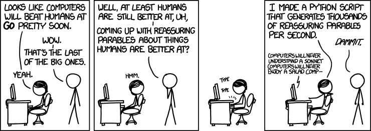
Wrap-up

Search

Search operates over models of the world (which might be observed online)

Agents do not try all possible plans
Planning is all “in simulation”
Search is only as good as the models are

Adversarial search

In two-player, discrete, deterministic, turn-taking zero-sum games with perfect information, the minimax algorithm can select optimal moves by a depth-first search in the game tree
Efficiency can be improved by using the alpha-beta search algorithm, which eliminates subtrees that are shown to be irrelevant.
Monte Carlo tree search evaluates states by playing out the game all the way to the end to see who won. This playout simulation is repeated multiple times. The evaluation is an average of the results.

xkcd

Q&A

Exercises

Definition sequence

Problem formulation must follow goal formulation.

Discuss that statement. Is it true or false? Why?

Problem formulation

Give a complete problem formulation for each of the following problems. Choose a formulation that is precise enough to be implemented.

There are six glass boxes in a row, each with a lock. Each of the first five boxes holds a key unlocking the next box in line; the last box holds a banana. You have the key to the first box, and you want the banana.
There is an n x n grid of squares, each square initially being either unpainted floor or a bottomless pit. You start standing on an unpainted floor square, and can either paint the square under you or move into an adjacent unpainted floor square. You want the whole floor painted.

Maze

Your goal is to navigate a robot out of a maze. It starts in the center of the maze facing north. You can turn the robot to face north, east, south, or west; direct the robot to move forward a certain distance (it will stop before a wall).

Formally define this problem as a search problem. How large is the state space?
In navigating a maze, the only place we need to turn is at the intersection of two or more corridors. Reformulate this problem using this observation. How large is the state space now?
From each point in the maze, we can move in any of the four directions until we reach a turning point, and this is the only action we need to do. Reformulate the problem using these actions. Do we need to keep track of the robot’s orientation now?
In our initial description of the problem we already abstracted from the real world. Name three such simplifications we made.

Solution notes

Figure 10: Solution note for the maze exercise

Problem statement

The center of the maze is at (0; 0), and the maze itself is a square from (-1;-1) to (1; 1).
Initial state: robot at coordinate (0; 0), facing North.
Goal test: either jxj > 1 or jyj > 1 where (x; y) is the current location.
Successor function: move forwards any distance d; change direction robot it facing.
Cost function: total distance moved.

The state space is infinitely large, since the robot’s position is continuous.

Reformulated problem statement

The state will record the intersection the robot is currently at, along with the direction it’s facing. At the end of each corridor leaving the maze we will have an exit node. We’ll assume some node corresponds to the center of the maze.

Initial state: at the center of the maze facing North.
Goal test: at an exit node.
Successor function: move to the next intersection in front of us, if there is one; turn to face a new direction.
Cost function: total distance moved.

There are 4n states, where n is the number of intersections.

Reformulated problem statement #2

Initial state: at the center of the maze.
Goal test: at an exit node.
Successor function: move to next intersection to the North, South, East, or West.
Cost function: total distance moved.

We no longer need to keep track of the robot’s orientation since it is irrelevant to predicting the outcome of our actions, and not part of the goal test. The motor system that executes this plan will need to keep track of the robot’s current orientation, to know when to rotate the robot.

Abstractions

State:

Ignoring the height of the robot off the ground, whether it is tilted off the vertical.
The robot can face in only four directions.
Other parts of the world ignored: possibility of other robots in the maze, the weather in the Caribbean.

Action:

We assumed all positions we safely accessible: the robot couldn’t get stuck or damaged.
The robot can move as far as it wants, without having to recharge its batteries.
Simplified movement system: moving forwards a certain distance, rather than controlled each individual motor and watching the sensors to detect collisions.

Concepts

Explain in your own words the following terms:

Zero-sum
Terminal test
Minimax value
Selection policy
Playout policy
Monte Carlo tree
Back-propagation

MINIMAX

Explain if the MINIMAX algorithm is complete and optimal.

Can it be beaten by an opponent playing suboptimally? Why (not)?

Come up with a game tree in which MAX will beat a suboptimal MIN.

Solution notes

Completeness

In two-player, discrete, deterministic, turn-taking zero-sum games with perfect information, the MINIMAX algorithm can select optimal moves by a depth-first emuration, the algorithm is also guaranteed to find a solution when there is one.

The algorithm performs a complete depth-first exploration of the game tree. If the maximum depth of the tree is \(m\) and there are \(b\) legal moves at each point, then the time complexity is \(O(b^m)\) for an algorithm that generates all actions at once, or \(O(m)\) for an algorithm that generates actions on at a time. The exponential complexity makes MINIMAX impractical for complex games. MINIMAX does, however, serve as a basis for the mathematical analysis for games. By approximating the minimax analysis in various ways, we can derive more practical algorithms.

Suboptimally play

If MIN does not play optimally, then MAX will do at least as well as against an optimal player, possibly better.

Pruning

Read the note about pruning (and consult Russel and Norvig (2022) if necessary).

Explain in your own words, under what conditions a subtree is skipped using Alpha-beta pruning.

Draw an example (game search tree, 3 levels depth).

Literature

Russel, Stuart, and Peter Norvig. 2022. Artificial Intelligence: A Modern Approach. Harlow: Pearson Education.

Footnotes

An atomic representation is one in which each state is treated as a black box with not internal structure, meaning the state either does or does not match what you’re looking for.
Problem formulation is specifically about defining the formal components of a search problem (state space, initial state, goal state, actions, etc.) — it’s about translating a real-world problem into the specific mathematical structure needed for search algorithms.
A state is a situation that an agent can find itself in.
Expressed by a graph whose nodes are the set of all states, and whose links are actions that transform one state into another
Can be a single goal state, a small set of alternative goal states, or a property that applies to many states (e.g, no dirt in any location)
First-in-first-out (FIFO) queue first pops the node that was added to the queue first
Last-in-first-out queue (LIFO; also known as a stack) pops first the most recently added node
First pops the node with the minimum costs according to \(f(n)\)
Reading recommendation
The average utility is guided by the selection policy.
For games with binary outcomes, average utility equals win percentage
Playout policies biases the moves toward good ones. For Go and other games, playout policies have been successfully learned from self-play by using neural networks. Sometimes also game-specific heuristics are used (e.g., take the corner square in Othello)