Introduction
Limits of traditional programming
Traditional programming approaches fail at tasks that humans find effortless.
For instance:
- Recognizing handwritten digits: Each “3” looks different, yet we instantly recognize the pattern
- Understanding context: “The bank” could refer to a financial institution or a river’s edge
- Learning from examples: We don’t need explicit rules to recognize new instances
Traditional programming relies on explicit rules and algorithms. For image recognition, you’d need to write code that handles every possible variation of how a digit could be drawn - different angles, sizes, writing styles, and lighting conditions. This quickly becomes intractable.
Human brains, however, excel at pattern recognition through learning from examples. We see many instances of the digit “3” and somehow extract the underlying pattern without being given explicit rules about what makes a “3” a “3”.
This paradox - tasks that are trivial for biological intelligence but nearly impossible for traditional programming - led to the development of neural networks and machine learning approaches that attempt to mimic how biological systems learn from data.
Recap: machine learning
Traditional programming:
\(Input + Program \rightarrow Output\)
Machine learning:
\(Input + Output \rightarrow Program\)
Differences
- Instead of writing explicit rules, we provide examples (training data)
- The machine learns patterns from these examples
- The resulting model can then make predictions on new, unseen data
Traditional programming requires us to understand and explicitly code the relationship between inputs and outputs. For complex tasks like image recognition, this becomes impossible because we can’t enumerate all the rules.
Machine learning flips this paradigm: we provide many examples of inputs paired with their correct outputs, and let the algorithm discover the underlying patterns. This is particularly powerful for tasks where the rules are too complex to code explicitly or where we don’t fully understand the underlying mechanisms ourselves.
The key insight is that many intelligent behaviors can emerge from relatively simple learning rules applied to large amounts of data, rather than requiring explicit programming of complex behaviors. This observation connects to the foundational work on neural networks by Rumelhart et al. (1986) and the theoretical foundations of universal approximation (Cybenko, 1989; Hornik et al., 1989).
Neural networks
Introduction
Neural networks solve problems that traditional programming cannot handle:
- Pattern recognition in noisy, variable data
- Decision making with incomplete information
- Automation of complex cognitive tasks
- Scaling human-like judgment to massive datasets
The beauty of neural networks lies in their universality - the same basic architecture that recognizes handwritten digits can be adapted to recognize faces, translate languages, or play games. This is because they learn to detect increasingly complex patterns through multiple layers of simple operations.
Understanding neural networks isn’t about memorizing mathematical formulas — it’s about recognizing when and how this technology can create business value. Neural networks excel in situations where:
Rules are hard to specify: Try writing explicit rules for recognizing the digit “3” across thousands of different handwriting styles. Traditional programming would require an impossibly complex set of if-then statements.
Human expertise is expensive to scale: A human can easily recognize digits, but hiring humans to process millions of documents isn’t feasible. Neural networks can replicate human-like pattern recognition at machine speed and scale.
Data is abundant but messy: Real-world data rarely fits neat categories. Neural networks can find patterns in noisy, incomplete, or variable data that would break traditional algorithms.
Adaptability is crucial: Business environments change constantly. Neural networks can be retrained on new data, allowing systems to adapt to changing conditions without complete reprogramming.
What is a neuron?
A neuron
receives inputs → weights them → sums up → activates
- This number is called the activation of the neuron
- High activation (close to 1.0) = neuron is “firing” or “lit up”
- Low activation (close to 0.0) = neuron is inactive
- Think of it as how excited the neuron is about a particular feature
The neuron is the fundamental computational unit that makes neural networks possible. While inspired by biological neurons, artificial neurons are much simpler mathematical functions. Understanding this building block is crucial because the entire network’s behavior emerges from millions of these simple operations.
Receiving inputs: Each neuron receives numerical values from the previous layer. In the first layer, these might be pixel intensities (0 for black, 1 for white). In deeper layers, these are the outputs of neurons from the previous layer.
Weighting inputs: Each connection has a “weight” - a number that determines how much influence that input has. Positive weights amplify the signal, negative weights suppress it, and weights near zero essentially ignore that input. These weights are the “knowledge” the network learns.
Summing: The neuron calculates a weighted sum: (input₁ × weight₁) + (input₂ × weight₂) + … + bias. The bias is like a threshold - it shifts the activation point of the neuron.
Activation function: The sum gets passed through a function (like sigmoid or ReLU) that determines the neuron’s output. This introduces non-linearity, allowing the network to learn complex patterns rather than just linear relationships.
Why this design works:
- Simplicity: Each neuron does something very simple, making the system robust and parallelizable
- Composability: Simple operations combine to create complex behaviors
- Differentiability: The mathematical smoothness allows for efficient learning algorithms
- Biological inspiration: While simplified, this captures key aspects of how biological neurons process information
The magic happens when thousands of these simple units work together in layers, each learning to detect different aspects of the input pattern.
Real neurons in the brain can be in various states of activation - they can fire action potentials at different rates, or remain quiet. The artificial neuron is a dramatic simplification, reducing this complex behavior to a single number between 0 and 1.
This simplification is intentional: by abstracting away the biological complexity, we can focus on the computational principles. The key insight is that neurons can represent information through their level of activation, and that these activations can be combined and transformed through networks to process complex information.
While the biological brain is vastly more complex, this simplified model has proven remarkably effective for a wide range of tasks, suggesting that some aspects of intelligence can emerge from relatively simple computational units arranged in the right structure.
Network architecture

The hierarchical organization of neural networks mirrors how human visual processing works, and this parallel isn’t coincidental — it’s one of the key insights that makes deep learning so powerful.
Connections between neurons
Each connection between neurons has a weight (positive or negative) — a number that gets adusted during learning.
- Positive weight: If the first neuron fires, it encourages the second neuron to fire
- Negative weight: If the first neuron fires, it discourages the second neuron from firing
- Bias: A constant added to shift when the neuron should activate

Weight mechanics
Positive vs. negative weights:
- Positive weights act like “encouragers” - when the input neuron is active (high value), it pushes the receiving neuron toward activation
- Negative weights act like “inhibitors” - when the input neuron is active, it pushes the receiving neuron toward inactivity
- Zero weights mean the connection is effectively ignored
Weight magnitude:
- Large positive weights create strong encouraging connections
- Large negative weights create strong inhibitory connections
- Small weights (near zero) have minimal influence
- The network learns which connections should be strong and which should be weak
This weighted sum with bias is the fundamental computation in neural networks. The weights determine how much influence each input has on the output, while the bias determines the baseline level of activation.
The sigmoid function \(\sigma(x) = \frac{1}{1 + e^{-x}}\) serves as a “squashing” function that ensures the output stays between 0 and 1, regardless of how large or small the weighted sum becomes. This is crucial for maintaining the “activation” interpretation of neuron outputs. Other activation functions commonly used are tanh, relu, and leaky relu.
The bias is particularly important because it allows the neuron to fire even when all inputs are zero, or to require a higher threshold before firing. Without bias, neurons could only learn patterns that pass through the origin, severely limiting the network’s expressiveness.
Understanding this computation is key to grasping how neural networks work: each neuron computes a weighted combination of its inputs, adds a bias, and applies a nonlinear function to produce its output. This forms the basis of the backpropagation algorithm developed by Rumelhart et al. (1986).
This perspective - viewing neural networks as complex mathematical functions - is crucial for understanding their power and limitations. The Universal Approximation Theorem (Cybenko, 1989; Hornik et al., 1989) tells us that neural networks with sufficient hidden units can approximate any continuous function to arbitrary accuracy.
The weights and biases represent the “knobs and dials” that can be adjusted to make the network compute any function we want (within the constraints of the architecture). Training is the process of finding the right setting for these parameters.
The power of neural networks comes from this massive number of adjustable parameters, which allows them to learn complex patterns in data. However, this also presents challenges: how do we find the right values for all these parameters? This is where the learning algorithms come in.
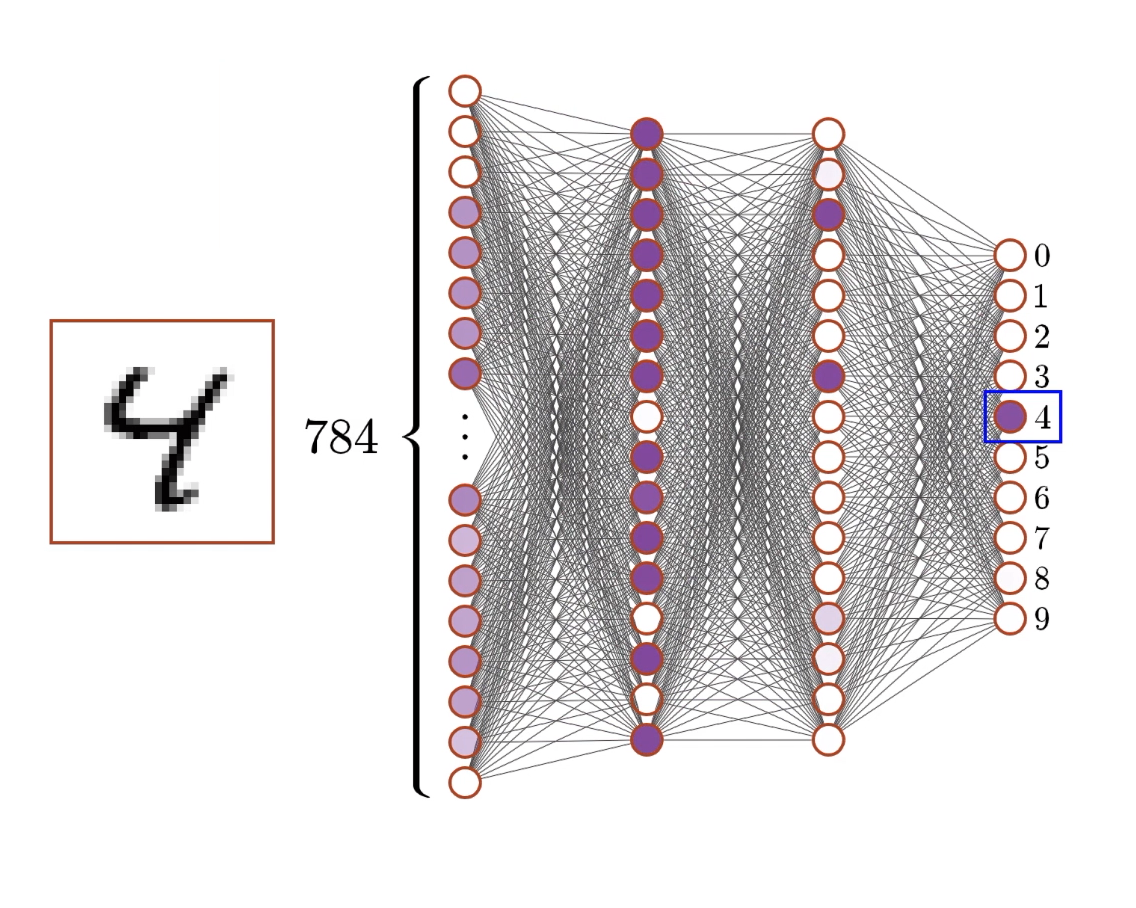
Example: digit recognition
Example architecture for detecting digits of the MNIST dataset1:
28×28 pixels → Neural Network → 10 probabilities
- Input layer: 784 neurons (28×28 pixels)
Each neuron represents one pixel’s brightness (0.0 = black, 1.0 = white) - Hidden layers: 2 layers, 16 neurons each
These learn to detect patterns and features - Output layer: 10 neurons Each represents confidence for digits 0-9
The architecture of our digit recognition network represents a carefully designed pipeline for transforming raw pixel data into digit classifications. Let’s understand why this specific structure makes sense:
Input layer (784 neurons):
- Each neuron represents one pixel in the 28×28 image
- Values range from 0 (black) to 1 (white), representing grayscale intensity
- This layer doesn’t perform computation - it just holds the input data
- 784 inputs might seem like a lot, but images require this level of detail to preserve important patterns
Hidden layer 1 (16 neurons):
- This is where the real pattern detection begins
- Each of these 16 neurons receives input from all 784 pixels
- With 784 inputs × 16 neurons = 12,544 weights (plus 16 biases)
- These neurons learn to detect fundamental features like edges, curves, and basic shapes
- 16 neurons is relatively small - real networks often use hundreds or thousands
Hidden layer 2 (16 neurons):
- Each neuron connects to all 16 neurons from the previous layer
- 16 inputs × 16 neurons = 256 weights (plus 16 biases)
- These neurons combine the basic features into more complex patterns
- They might detect things like “loop at top” or “vertical line on left”
Output layer (10 neurons):
- One neuron for each possible digit (0, 1, 2, …, 9)
- 16 inputs × 10 neurons = 160 weights (plus 10 biases)
- Each neuron’s activation represents the network’s confidence that the input image shows that particular digit
- The highest activation typically indicates the network’s “guess”
Total Parameters:
- Weights: 12,544 + 256 + 160 = 12,960
- Biases: 16 + 16 + 10 = 42
- Total: 13,002 adjustable parameters
This seems like a lot, but it’s actually quite modest by modern standards. Large language models can have billions of parameters. The key insight is that all these parameters work together to create a flexible function that can map any 28×28 image to a probability distribution over the 10 digit classes.
Learning
The learning problem
Goal: Find the values of all k parameters that make the network classify digits correctly.
Challenge: This is a k-dimensional optimization problem!
(In our digit example it is 13,002-dimensional)
We need a systematic way to:
- Measure how “wrong” the network currently is
- Determine which parameters to adjust
- Make small improvements iteratively
Optimizing in 13,002 dimensions is conceptually challenging for humans to visualize, but mathematically tractable. Each dimension represents one parameter (weight or bias) in the network.
The challenge is immense: with 13,002 parameters, there are potentially infinite ways to set these values. Most combinations will perform poorly, and we need to find the tiny subset that actually works well for digit recognition.
Traditional optimization approaches (like trying random combinations or exhaustive search) would take longer than the age of the universe. We need smarter approaches that can navigate this high-dimensional space efficiently.
The key insight is that we can use calculus — specifically derivatives — to determine the direction of steepest improvement. This allows us to make educated guesses about how to adjust parameters rather than random exploration.
Cost functions
For a single training example, if the network outputs \((a_0, a_1, ..., a_9)\) but the correct answer is digit \(k\):
Desired output: \((0, 0, ..., 1, ..., 0)\) (1 in position \(k\), 0 elsewhere)
Cost for this example:
\(C = \sum_{j=0}^{9} (a_j - y_j)^2\)
where \(y_j\) is the desired output for neuron \(j\).
The squared error cost function has several nice properties:
- Always positive: Squared terms ensure the cost is never negative
- Smooth and differentiable: We can compute gradients needed for optimization
- Penalizes large errors more: A network that’s very wrong gets penalized more than one that’s slightly wrong
- Zero when perfect: Cost is exactly 0 when the network output matches the desired output perfectly
For digit recognition, if the correct answer is “3”, we want:
- Output neuron 3 to have activation close to 1.0
- All other output neurons to have activation close to 0.0
The cost function measures how far we are from this ideal. When the network is confident and correct, the cost is low. When the network is uncertain or wrong, the cost is high.
Alternative cost functions exist (like cross-entropy), but squared error is conceptually simpler and works well for educational purposes.
Gradient descent
Intuition: Imagine the cost function as a landscape with hills and valleys. We want to find the lowest valley (minimum cost).
Gradient descent algorithm:
- Compute the gradient (direction of steepest increase in cost)
- Move in the opposite direction (direction of steepest decrease)
- Take small steps to avoid overshooting
- Repeat until you reach a minimum
The landscape metaphor is powerful but limited. In 13,002 dimensions, we can’t visualize the actual landscape, but the mathematical principles remain the same.
Key insights about gradient descent:
Local vs global minima: Like a real landscape, the cost function may have multiple valleys. Gradient descent finds a local minimum (nearby valley) but might miss the global minimum (deepest valley overall).
Learning rate: This is a crucial hyperparameter:
- Too large: We might overshoot and oscillate around the minimum
- Too small: Progress is very slow, and we might get stuck
- Just right: Steady progress toward a minimum
High-dimensional intuition: In high dimensions, most points are neither maxima nor minima, but saddle points. This actually helps optimization because there are usually many directions that lead downhill.
Why it works: Even though we can’t visualize 13,002-dimensional space, the mathematical guarantee is that moving in the negative gradient direction will decrease the cost (at least for small steps).
Backpropagation
Challenge: How do we compute the gradient of the cost function with respect to all k parameters efficiently?
Backpropagation algorithm:
- Forward pass: Run the network on a training example to get predictions
- Compute cost: Compare predictions to correct answers
- Backward pass: Use the chain rule2 to compute how each parameter affects the cost
- Update parameters: Adjust each parameter in the direction that reduces cost
This elegant algorithm, formalized by Rumelhart et al. (1986), makes training deep networks computationally feasible (Sanderson, 2017b).
Backpropagation is essentially an efficient application of the chain rule from calculus. The key insight is that we can compute gradients by working backwards through the network.
Forward Pass Example: Input → Layer 1 → Layer 2 → Output → Cost
Backward Pass: Cost → ∂Cost/∂Output → ∂Cost/∂Layer2 → ∂Cost/∂Layer1 → ∂Cost/∂Weights
For each parameter, we ask: “If I change this parameter by a tiny amount, how much does the cost change?” The chain rule lets us compute this efficiently by decomposing the influence into steps.
Think of it as tracing cause and effect:
- How did weight W affect neuron N?
- How did neuron N affect the layer’s output?
- How did the layer’s output affect the final prediction?
- How did the final prediction contribute to the error?
Why “Backpropagation”?: We propagate the error backwards through the network. Starting from the final cost, we compute how much each layer contributed to that cost, then how much each neuron contributed, and finally how much each weight contributed.
This algorithm is remarkably efficient: computing the gradient for all parameters takes roughly the same computational time as computing the network’s output itself. This efficiency made training deep networks practical (Sanderson, 2017b).
Learning loop
- Start with random weights
- Make a prediction (forward pass)
- Measure the error
- Trace back to find responsible weights (backpropagation)
- Adjust weights to reduce error
- Repeat with the next example
Through millions cycles, the network gradually learns to recognize even complex patterns.
The remarkable thing is that complex behaviors (like recognizing handwriting) emerge from this simple process of error correction.
This transformation from random guesses to intelligent recognition happens purely through this iterative process of prediction, error measurement, and weight adjustment. No human explicitly programs the features - the network discovers these patterns automatically through experience.
Using mini-batches for training
There are three main approaches to gradient descent:
Batch Gradient Descent: Use all training examples to compute gradient
- Pros: Most accurate gradient estimate
- Cons: Very slow for large datasets, memory intensive
Stochastic Gradient Descent (SGD): Use one example at a time
- Pros: Fast updates, can escape local minima due to noise
- Cons: Very noisy, unstable convergence
Mini-batch SGD: Use small batches (typically 16-256 examples)
- Pros: Good balance of speed and stability
- Cons: Requires tuning batch size
Mini-batches provide several advantages:
- Computational efficiency: Modern hardware (GPUs) is optimized for parallel processing of batches
- Better gradient estimates: Averaging over multiple examples reduces noise
- Memory efficiency: Process data in chunks rather than loading everything
- Regularization effect: The noise from mini-batching can help escape poor local minima
The choice of batch size is another hyperparameter that affects training dynamics and final performance (Sanderson, 2017a).
Mini-batch stochastic gradient descent:
- Shuffle the training data randomly
- Divide into small batches (e.g., 32 examples per batch)
- For each batch:
- Compute gradients for all examples in the batch
- Average the gradients across the batch
- Update parameters using the averaged gradient
- Repeat for many epochs3
Key insights
- Neural networks excel when the data has many features and complex relationships between them (e.g., images, text, customer behavior, financial markets).
- Neural networks can find patterns in this complexity that would be impossible to detect manually or with simpler algorithms.
- Neural networks are remarkably robust to noisy, imperfect data (e.g., missing values, measurement errors, outliers) because they learn statistical patterns rather than requiring perfect data.
- Neural networks often improve with more data, unlike many traditional methods that plateau.
- Business environments change constantly. Neural networks can be retrained on new data to.
Transformers
From images to language
The challenge
Key differences between images and text:
- Images has fixed size (e.g., 28×28 pixels) and spatial relationships matter
- Text has variable length, sequential relationships matter, and context is crucial
- Word meaning depends heavily on surrounding words
- “The bank was flooded” vs “I went to the bank”
- “model” in “machine learning model” vs “fashion model”
We need architectures designed specifically for sequential data with long-range dependencies.
Standard neural networks, like our digit classifier, have limitations for language:
- Fixed Input Size: Traditional networks expect fixed-size inputs, but sentences have varying lengths
- No Sequential Understanding: Standard networks treat input positions independently - they can’t understand that word order matters
- No Long-Range Dependencies: Information from early in a sentence might be crucial for understanding words much later
Early attempts to solve this included:
- Recurrent Neural Networks (RNNs): Process sequences one word at a time, but suffer from vanishing gradients for long sequences
- Convolutional Networks: Good for local patterns but struggle with long-range dependencies
- LSTM/GRU: Better than RNNs but still fundamentally sequential and slow to train
The breakthrough came with Transformers (Vaswani et al., 2017), which solved these problems through a fundamentally different approach: attention mechanisms that allow every word to directly interact with every other word in the sequence.
What is a Transformer?
A transformer is a neural network architecture specifically designed for processing sequences.
The attention mechanism is the key innovation — it allows every element in the sequence to “attend to” every other element.
The Transformer architecture, introduced in the landmark 2017 paper “Attention Is All You Need” (Vaswani et al., 2017), revolutionized natural language processing. The key insight was that attention mechanisms could replace recurrent and convolutional layers entirely.
Before transformers, most language models were based on RNNs or CNNs, which processed sequences step-by-step or with limited context windows. This made them slow to train and limited in their ability to capture long-range dependencies.
The attention mechanism allows for:
- Parallel processing: All positions in a sequence can be processed simultaneously
- Long-range dependencies: Any word can directly attend to any other word, regardless of distance
- Interpretability: We can visualize what the model is “paying attention to”
The impact has been enormous:
- GPT (Generative Pre-trained Transformer) family: GPT-1, GPT-2, GPT-3, GPT-4
- BERT: Bidirectional transformer for understanding tasks
- T5: Text-to-text transfer transformer
- and hundreds of other transformer-based models
The name “Transformer” comes from its ability to transform input sequences into output sequences through the attention mechanism.
Context is everything
Consider these sentences:
- “The tower was very tall”
- “The Eiffel tower was very tall”
The word “tower” should mean different things in different contexts:
- First case: Generic tower
- Second case: Specific famous landmark in Paris
Attention mechanism allow context words to update the meaning of other words.
Tokens and embeddings
Tokenization means that text is broken down into small chunks called tokens — a crucial preprocessing step that bridges human language and machine processing.
- “To date, the cleverest thinker of all time was…”
- Becomes: [“To”, “date”, “,”, “the”, “cle”, “ve”, “rest”, “thinker”, “of”, “all”, “time”, “was”, “…”]
Each token gets converted to a high-dimensional vector (e.g., 12,288 dimensions for GPT-3) — so called embedding vectors
- Similar tokens get similar vectors
- These vectors capture semantic meaning
This vector representation is what the transformer actually processes - it never sees raw text, only these numerical vectors (Sanderson, 2024a).
Word Embeddings
Directions in embedding space can encode semantic relationships.
Examples:
- Gender direction: “king” - “man” + “woman” ≈ “queen”
- Plurality direction: “cat” - “cats” captures singular vs plural
- Country-capital: “Germany” - “Berlin” + “France” ≈ “Paris”
The embedding layer learns to place semantically related words close together in the vector space.
Word embeddings reveal that meaning has geometric structure. This isn’t just a mathematical curiosity - it reflects how language itself is structured:
Analogical reasoning — the famous “king - man + woman = queen” example shows that semantic relationships can be captured as vector operations. This suggests that certain directions in the embedding space consistently encode specific semantic properties.
Semantic clusters — words with similar meanings cluster together:
- Animals: “dog”, “cat”, “horse” are close to each other
- Colors: “red”, “blue”, “green” form another cluster
- Countries: “France”, “Germany”, “Italy” cluster together
Hierarchical structure — the space can capture hierarchies:
- “Animal” might be close to “Dog”, “Cat”, etc.
- “Mammal” might be between “Animal” and “Dog”
Cultural and linguistic biases — embeddings can capture societal biases present in training data:
- Occupational gender stereotypes
- Racial or cultural associations
- This is both a feature (capturing human-like associations) and a bug (perpetuating unfair biases)
Training process — These embeddings aren’t hand-crafted but learned from data. The model discovers these geometric relationships by seeing how words are used together in context (Sanderson, 2024a).
Attention
Rather than having fixed embeddings for each word, attention allows the embedding to be dynamically updated based on what other words are present in the context. This creates context-sensitive representations that can capture these nuanced meanings.
Single-head attention
Goal: Update the embedding of some word on the context of that word.
Three key matrices (learned during training)4:
- Query matrix \(W_Q\) indicates what types of context each word typically needs
- Key matrix \(W_K\) indicates what types of context each word can provide
- Value matrix \(W_V\) indicates what information to actually pass
Process:
- Compute attention scores between words
- Create weighted combinations of information
- Update embeddings based on relevant context
Example
Let’s trace how attention helps resolve the ambiguity of “bank” (financial institution vs. riverbank).
The target word is “bank” (needs contextual disambiguation), the context word is “flooded”
The attention process
- Step 1: attention score:
“bank’s” query vector × “flooded’s” key vector = high similarity score
(the model has learned that water-related words are highly relevant for disambiguating “bank”) - Step 2: weighted information:
high attention score × “flooded’s” value vector = strong water/geography signal - Step 3: contextualized embedding:
original “bank” embedding + weighted “flooded” information = “riverbank” meaning
The ambiguity is resolved: we’re talking about a riverbank, not a financial institution
Multi-head attention
In reality different types of relationships matter simultaneously, such as
- Head 1 might focus on grammatical relationships (subject-verb agreement)
- Head 2 might focus on semantic relationships (synonyms, antonyms)
- Head 3 might focus on coreference (pronouns to their referents)
- Head 4 might focus on long-range dependencies (cause and effect)
Each head learns to specialize in different types of patterns and relationships.
GPT-3 example: 96 attention heads per layer × 96 layers = 9,216 total attention heads
Feed-forward networks (FFN)
After attention, each token passes through a FFN.
FFNs are the “thinking” components that sit between attention layers in transformers. While attention figures out what information to gather, FFNs decide what to do with that information.
Example:
- Attention: Given ‘bank’ and ‘flooded,’ I should focus on the flooding information
- FFN: Now that I know this is a flooded riverbank, I should activate concepts related to environmental damage and strengthen connections to geographic features
Following residual connections and layer normalization make deep transformers stable and trainable.
A residual connection means you add the input back to the output of a layer:
output = Layer(input) + input
Or more specific:
- After attention layer:
contextualized_embedding = attention(original_embedding) + original_embedding - After FFN layer:
final_output = ffn(contextualized_embedding) + contextualized_embedding
Without residual connections: Information can get “lost” or distorted as it passes through many layers With residual connections: The original information is always preserved and combined with the processed version.
Layer normalization standardizes the values within each embedding vector to have mean close to 0 and standard deviation close to 1.
Unembedding
From vectors back to text.
The unembedding process is how transformers convert their internal vector representations back into text predictions. It’s the crucial final step that makes language generation possible.
Process
Example
- Context processing: “The capital of France is” → final vector
- Unembedding: Vector × W_U → raw scores for all 50,257 tokens
- Temperature scaling: Divide scores by temperature
- Softmax: Convert to probability distribution
- Sampling: Choose next token based on probabilities
Transformer architecture overview
Key principle: Information flows through many layers of attention and processing (i.e., built through deep learning), allowing complex reasoning to emerge.
- Tokenization + embedding: Text → Vectors
- Attention blocks: Vectors communicate and update based on context
- Feed-forward layers: Independent processing of each vector
- Many layers: Alternate attention and feed-forward (e.g., 96 layers in GPT-3)
- Unembedding: Final vector → Probability distribution over next tokens
Training
Training process
No explicit labels needed — the text itself provides the training signal.
Next-token prediction seems simple but is remarkably powerful (Radford et al., 2019):
- Implicit learnings comprise grammar, facts, reasoning, coding and patterns
- More training data exposes the model to more patterns and knowledge (scale effects)
- More training time allows better optimization of the massive parameter space
- Training requires immense training infrastructure (GPT-3 training cost ~$4.6 million in compute)
Emergent capabilities
As models scale up, they develop capabilities that weren’t explicitly programmed:
- Few-shot learning: Learn new tasks from just a few examples
- Chain-of-thought reasoning: Break complex problems into steps
- Code generation: Write and debug programs
- Mathematical reasoning: Solve word problems and equations
- Creative writing: Generate stories, poems, and scripts
- Instruction following: Understand and execute complex commands
Complex intelligence seem to emerge from the simple objective of predicting the next word.
Limitations and Challenges
Despite their impressive capabilities, current language models have significant limitations:
- Hallucination: Generate plausible-sounding but false information
- Lack of true understanding: May memorize patterns without genuine comprehension
- Inconsistency: May give different answers to the same question
- Training data bias: Reflect biases present in internet text
- No learning from interaction: Can’t update their knowledge from conversations
- Computational requirements: Expensive to train and run
Further reads
Please check the resources provided by 3Blue1Brown on the basics of neural networks, and the math behind how they learn.
Exercises
Neural network architecture
Design a neural network for classifying emails as spam or not spam. Specify:
- Input representation: How would you convert an email into numbers?
- Output: How would you interpret the network’s output?
- Training data: What kind of examples would you need?
Discuss the advantages and challenges of this approach compared to rule-based spam filtering.
Input representation options
- Bag of words: Count frequency of each word in vocabulary (e.g., 10,000 input neurons)
- TF-IDF: Weight word frequencies by inverse document frequency
- Word embeddings: Use pre-trained embeddings and average/pool them
- Character-level: Represent emails as sequences of characters
Output interpretation
- Single output neuron with sigmoid activation
- Value close to 1 = spam, close to 0 = not spam
- Use threshold (e.g., 0.5) for binary classification
Training data requirements
- Thousands of labeled emails (spam/not spam)
- Balanced dataset or careful handling of class imbalance
- Diverse examples covering different types of spam
- Regular updates as spam techniques evolve
Advantages over rules
- Automatically learns patterns from data
- Adapts to new spam techniques
- Can detect subtle combinations of features
- Less manual maintenance required
Challenges
- Requires large labeled datasets
- Can be fooled by adversarial examples
- Black box - hard to understand why decisions are made
- May learn biases from training data
Attention mechanism
Consider the sentence: “The red car that John bought yesterday broke down on the highway.”
- Identify relationships: What words should attend to each other strongly?
- Multiple heads: Design 3 different attention heads that focus on different types of relationships.
- Context update: How should the embedding of “car” change after processing this sentence?
Strong attention relationships
- “red” → “car” (adjective modifies noun)
- “car” → “broke” (subject-verb relationship)
- “that” → “car” (relative pronoun reference)
- “John” → “bought” (subject-verb)
- “bought” → “car” (verb-object)
- “yesterday” → “bought” (temporal modifier)
- “broke” → “highway” (location context)
Three attention head types
- Grammatical relationships
- Focus on syntactic dependencies
- “car” attends to “broke” (subject-verb)
- “John” attends to “bought” (subject-verb)
- Helps with grammatical consistency
- Modification relationships
- Focus on descriptive relationships
- “red” attends to “car”
- “yesterday” attends to “bought”
- Captures qualitative and temporal information Coreference and long-range
- Focus on pronoun resolution and distant relationships
- “that” attends to “car”
- “broke” attends back to “car” (long-range subject)
- Handles complex sentence structure
Car embedding updates
- Initial: Generic car concept
- After “red”: Specific colored vehicle
- After “John bought”: Particular car owned by John
- After “yesterday”: Recently purchased car
- After “broke”: Problematic/unreliable vehicle
- Final representation: John’s recently-purchased red car with reliability issues
Transformer training
You’re training a small transformer to complete simple mathematical expressions like “2 + 3 = ?”
- Tokenization: How would you represent mathematical expressions as tokens?
- Training objective: What would be your training data and loss function?
- Challenges: What difficulties might arise, and how would you address them?
- Evaluation: How would you test if the model truly “understands” arithmetic?
Tokenization strategies
- Character-level: [‘2’, ‘+’, ‘3’, ‘=’, ‘?’] - simple but may struggle with multi-digit numbers
- Number tokens: [‘2’, ‘+’, ‘3’, ‘=’, ‘?’] - treat each number as atomic token
- BPE encoding: Learn subword patterns for larger numbers
- Special tokens: [NUM_2, OP_PLUS, NUM_3, OP_EQUALS, MASK]
Training data and objective
- Data generation: Automatically generate arithmetic problems
- Simple: “1 + 1 = 2”, “5 - 3 = 2”
- Complex: “12 × 7 = 84”, “100 ÷ 4 = 25”
- Objective: Next token prediction
- Input: “2 + 3 =”
- Target: “5”
- Loss function: Cross-entropy loss on predicted vs. true next token
Challenges and solutions
- Out-of-distribution numbers: Train on wide range, test generalization
- Order of operations: Include parentheses: “(2 + 3) × 4 = 20”
- Digit-by-digit vs. holistic:
- Problem: Might predict “1” then “2” for “12” without understanding the full number
- Solution: Use single tokens for numbers or special training techniques
- Systematic vs. memorization: Risk of memorizing rather than learning arithmetic
Evaluation strategies
- Held-out test set: Numbers and operations not seen in training
- Systematic generalization: Can model handle larger numbers than in training?
- Error analysis: Do mistakes follow patterns that suggest understanding vs. memorization?
- Compositional tests: Can model handle combinations like “2 + 3 × 4”?
- Ablation studies: How does performance vary with model size, training data size?
Evidence of understanding
- Generalization: Correct answers on unseen number combinations
- Consistency: Same answer for equivalent expressions (“2+3” vs “3+2”)
- Error patterns: Mistakes that make mathematical sense (off by one) vs. random errors
- Intermediate reasoning: Model generating step-by-step solutions
Ethics and AI safety
A company wants to deploy a large language model for automated customer service. Consider the following scenario:
Situation: The AI occasionally provides incorrect information about product returns, leading to customer frustration and potential financial losses.
- Identify risks: What are the potential harms from this deployment?
- Mitigation strategies: How could the company reduce these risks?
- Monitoring: What metrics should they track to ensure safe operation?
- Human oversight: When should humans intervene in the AI’s responses?
Potential risks and harms:
- Customer harm: Incorrect return information could cost customers money
- Brand damage: Poor AI interactions damage company reputation
- Legal liability: Company might be liable for AI’s incorrect advice
- Bias amplification: AI might treat different customer groups unfairly
- Escalation: Frustrated customers might become abusive toward human agents
- Over-reliance: Customers might trust AI advice over written policies
Mitigation strategies:
- Knowledge grounding: Connect AI to authoritative policy databases
- Confidence thresholds: Route uncertain queries to human agents
- Response templates: Limit AI to pre-approved response patterns for critical information
- Fact verification: Cross-check AI responses against official policies
- User education: Clearly indicate when users are interacting with AI
- Fallback mechanisms: Easy escalation path to human support
Monitoring metrics:
- Accuracy rates: Percentage of correct responses on return policy queries
- Customer satisfaction: Post-interaction surveys and ratings
- Escalation rates: How often customers request human assistance
- Error types: Categorize and track different kinds of mistakes
- Bias metrics: Performance across different customer demographics
- Business impact: Track correlation between AI interactions and returns/complaints
Human oversight triggers:
- High-stakes queries: Expensive items, complex return situations
- Uncertainty indicators: When AI confidence scores are low
- Customer frustration: Detecting anger or confusion in customer messages
- Policy exceptions: Cases requiring
Temperature and text generation
You are working with a language model that produces the following raw scores (logits) for the next token after the prompt “The weather today is”:
Raw scores: [sunny: 2.0, cloudy: 1.8, rainy: 1.2, snowy: 0.8, windy: 0.6]
- Calculate probabilities: compute the probability distribution using softmax for temperatures T = 0.5, T = 1.0, and T = 2.0.
\(P(token_i) = \frac{e^{score_i/T}}{\sum_j e^{score_j/T}}\)
- Analyze the effects:
- Which temperature setting would be best for a weather report (factual, reliable)?
- Which would be best for creative writing (varied, interesting)?
- What happens as temperature approaches 0? As it approaches infinity?
- Practical implications:
- If you were building a chatbot for customer service, what temperature would you choose and why?
- How might you dynamically adjust temperature based on the type of response needed?
Probabilities
\(P(token_i) = \frac{e^{score_i/T}}{\sum_j e^{score_j/T}}\)
T = 0.5 (low/focused)
- sunny: \(e^{2.0/0.5} = e^4 = 54.6\)
- cloudy: \(e^{1.8/0.5} = e^{3.6} = 36.6\)
- rainy: \(e^{1.2/0.5} = e^{2.4} = 11.0\)
- snowy: \(e^{0.8/0.5} = e^{1.6} = 5.0\)
- windy: \(e^{0.6/0.5} = e^{1.2} = 3.3\)
Sum = 110.5
Probabilities: [0.49, 0.33, 0.10, 0.05, 0.03]
T = 1.0 (balanced)
- sunny: \(e^{2.0} = 7.4\)
- cloudy: \(e^{1.8} = 6.0\)
- rainy: \(e^{1.2} = 3.3\)
- snowy: \(e^{0.8} = 2.2\)
- windy: \(e^{0.6} = 1.8\)
Sum = 20.7
Probabilities: [0.36, 0.29, 0.16, 0.11, 0.09]
T = 2.0 (high/creative)
- sunny: \(e^{1.0} = 2.7\)
- cloudy: \(e^{0.9} = 2.5\)
- rainy: \(e^{0.6} = 1.8\)
- snowy: \(e^{0.4} = 1.5\)
- windy: \(e^{0.3} = 1.3\)
Sum = 9.8
Probabilities: [0.28, 0.25, 0.18, 0.15, 0.13]
Analysis of effects
- Weather report: T = 0.5 (focused on most likely/accurate predictions)
- Creative writing: T = 2.0 (more variety and unexpected choices)
- As T → 0: Distribution becomes deterministic (always picks highest score)
- As T → ∞: Distribution becomes uniform (all choices equally likely)
Practical implications
- Customer service chatbot: T = 0.3-0.7 (reliable, helpful responses)
- Dynamic adjustment:
- Factual questions: Low temperature
- Creative requests: High temperature
- Could analyze prompt content to auto-adjust
Key Insights
- Temperature is a crucial hyperparameter for controlling creativity vs. reliability
- Lower temperature = more predictable, higher accuracy
- Higher temperature = more diverse, creative outputs
- The choice depends entirely on the application and desired behavior
- Dynamic adjustment based on context can optimize user experience
Literature
Footnotes
The MNIST (Modified National Institute of Standards and Technology) dataset is a popular dataset used for training and testing image classification systems, especially in the world of machine learning. It contains 60,000 training images and 10,000 test images of handwritten digits.↩︎
For a visual explanation see 3blue1brown — Visualizing the chain rule and product rule↩︎
An epoch is one complete pass through the entire training dataset. During one epoch, the model sees every training example exactly once. Training might stop after a certain number of epochs or when performance plateaus.↩︎
During training by means of backpropagation, the attention matrices \(W_Q\), \(W_K\), and \(W_V\) learn patterns. Thus, these are essentially weights in the neural network — they’re learned parameters just like weights in any other layer.↩︎
An embedding dimension of 12,288 means each word/token is represented as a vector with 12,288 numbers. Each position captures some aspect of meaning - though not interpretable to humans.↩︎
A vocabulary size of 50,257 tokens means the model knows 50,257 different tokens (words, word pieces, punctuation, etc.).↩︎
High temperature → more random/creative; low temperature → more focused/deterministic↩︎